In machine learning and deep learning, cross entropy is used extensively as a loss function in a classification problem. In order to understand the it's intuition, we need to understand it's origin from an area of computer science called Information Theory.
In digital era, the main goal is to transfer the data reliably and efficiently from a sender to a recipient. We know that the transfer is done in bits. But the main problem is how to encode it. And most importantly how to know if that encoding is good or bad, OR how much unnecessary information that we are sending.
While sending a message, not all bits are useful. Claude Shannon proposed a way to measure to measure how efficient the transfer is in his paper that later became the foundation for Information theory.
What is Uncertainty factor reduction?
Let's just take an example of transmitting weather information from weather station to you. We consider few cases to understand the reduction in uncertainty factor with different weather states.
1. Weather being random with 2 states
In this case we assume that the weather can either be Sunny or Rainy with equal probability.
These are the probabilities that we are assuming prior to the transmission. If the weather station transmits that it is going to be rainy, then according to Shannon, they(weather station) reduced our uncertainty by a factor of 2.
It is very important to note that we are not trying to predict anything here. The probabilities are something that we assumed from the previous data( generally ) and we are receiving the forecast information from the weather station. All we are trying to do here is to measure how efficient the transfer is. It doesn't matter whether tomorrow that it is actually going to rain or not.
- One other way to interpret this is before the forecast we are only 50% certain, But we are 100% certain, that means, our certainty has increased from 50% to 100%, with a factor of 2.
- Another way to put this is as follows. We had 2 options out of which 1 is sunny and the other is rainy. We were not sure ( uncertain ) which we are going to receive from the weather station. After the forecast that it is going to be rainy, we are down to one option(rainy) from the available options(rainy and sunny). This is a reduction. Just like before we can calculate the reduction in our uncertainty as follows.
While calculating certainty factor, we are multiplying the factor because we want to measure by how much our certainty factor has increased.
Similarly, while calculating the uncertainty factor, there is a division because we want to calculate the factor by how much our uncertainty has reduced.
2. Weather being random with 8 possible states
In this example, let's just say the weather can be any of the 8 states say from sunny to rainy. And it is important to note that all are equally likely.
From the weather station, let's just say we received the forecast as . Now, let's just calculate the factor by which there is an increase in certainty or decrease in uncertainty.
-
certainty increased from to . i.e., from ( to )
-
Uncertainty decreased from 8 possible cases () to 1 case ().
3. Weather with 2 states ( But NOT Equally likely )
In this case we assume that there is 75% chance that the weather would be sunny and 25% chance that the weather would be rainy. In the previous two cases, the reduction factor is same (2 and 8 in first and second example respectively) irrespective of the forecast because the probabilities are same. Here, it is little different.
One other way to put this is by considering having 4 options out of which 3 options are sunny and one is rainy.
Because the probabilities are little different, the reduction in uncertainty factor or increase in certainty factor for sunny and rainy would be different.
3.1 Rainy
First, let's say that the weather station forecasted it as rainy. Before the forecast, we are only 25% sure that it is going to be rainy, but after the forecast, we are 100% sure.
- certainty increased from 25% to 100%
In other words, we were uncertain that which of the four cases are we gonna receive, but after the forecast, we know for sure that it would be rainy. So we were down from having 4 cases to 1.
- uncertainty decreased from 4 possible options to 1 option.
3.2 Sunny
If the forecast is sunny, we can calculate the increase in certainty or the decrease in uncertainty the same way as before. Here it is little tricky but if you understood the previous things, then it seems intuitive.
-
certainty increased from to
-
uncertainty decreased from 4 possible ( 3 sunny and 1 rainy ) options to 3 options( sunny ).
What about Information ?
So far we've been learning about the uncertainty factor, but what about the information. According to Shannon, transferring 1 bit means reducing the recipients uncertainty factor by 2. We will try to come up with a general notation below
| Reduction in Uncertainty by a factor | Information transferred in bits |
|---|---|
| 2 | 1 bit |
| 4 | 2 bits |
| 8 | 3 bits |
| .... | .... |
| ... | |
| f | bits |
And from above all three examples, the reduction factor is exactly inverse of probability that we assumed before the transmission. From this, we can write the ( useful ) information received as follows.
If the probability of an event happening is , then the (useful) information transferred to the recipient is .
We are calling the information transferred as useful because, sender might convey the same information in so many ways ( in bits ). If it is regarding weather, they can encode the information( each weather state) as a string where in each character is of 1 Byte. OR they can decide some character for each weather state and send that instead of whole string. Whatever the encoding it may be, according to Shannon, the useful number of bits, which we are calling information is negative logarithm of probability of that event, i.e., bits.
The number of bits that are being transmitted in a transmission on an average is nothing but entropy. The physics definition for this is that it is a measure of uncertainty or randomness, which makes sense.
Entropy
It is the average amount of useful information that is being transferred. Statistically, it is called as the expected information. And as mentioned before the probabilities are learned based on the past data.
Let's consider the case where we have the probability of weather being sunny is 75% and rainy is 25%. In this case the entropy is bits. i.e.,. Please use calculator to verify the same.
Entropy - Measure of Uncertainty?
It may be little confusing at first, but it actually tells you how un certain our events are. If the weather is same almost every day, say sunny, then the average amount of information that we get is not that much. In fact close to zero.
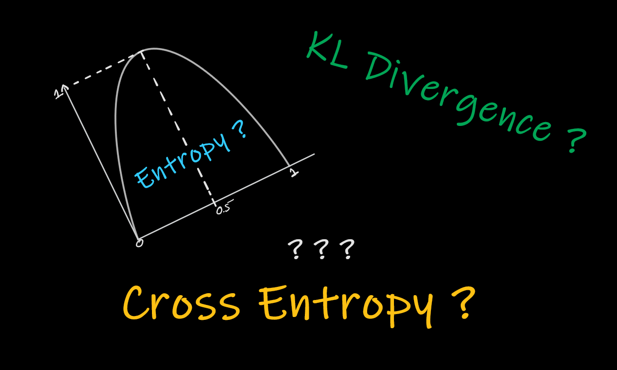
Below graph is for the Entropy when we have two events. Here the equation of Entropy is calculated as because the probabilities sums to 1 when there are two events.
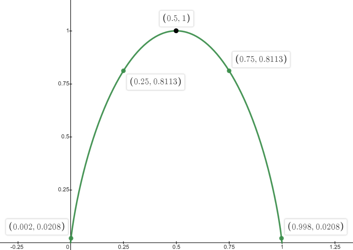
As we have only two events, if the probability of one event is high then the other event's probability would be low .
Low Entropy when events are certain
If we take the previous case as an example with two cases(sunny and rainy), If the weather is almost sunny like 95% of the time, irrespective of the forecast, the information is very low. You can observe the same in the graph as well. It makes sense intuitively too if you think about it. If someone tells you that that it would be sunny where it is sunny almost everyday (95%), On an average, you are not gonna get benefitted from that message.
High Entropy for uncertain events
Consider the case where weather is random everyday. An ideal case would be 50% - 50% for sunny and rainy. In such cases, whatever the message that you receive from the weather station, it would be so much useful on an average. And you can observe the same from the graph as well. the entropy is high.
Cross Entropy
Before going to discuss this, first we need to clear few things about Entropy.
-
For entropy, we were just calculating the ideal / useful information given just the probabilities, nothing else.
-
In all the above examples, all the events are dependent and their probabilities sums to 1. It is not true always. The events might be independent. The information that you get from a weather station is completely independent of the information that you get from a different source. As these are independent, we can just sum the information content from these two sources to get total Useful Information.
-
From source, , let's just say the events probabilities are , and the information is .
-
From source , say the events probabilities are , and the information is .
-
Total Information, .
-
This can be interpreted as all the events coming from a single source. The over all information(useful) is not gonna effect. All we need is a list of probabilities of the events to calculate the entropy.
-
What is cross-Entropy?
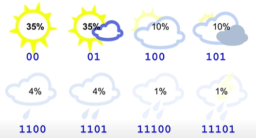
It is nothing but the average amount of information(in bits) in a transmission. Consider the following example where we encode all the events as 3 bits and assuming all the events are equally likely. In this case, Cross Entropy is 3 bits.
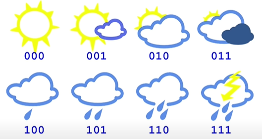
When we are encoding any information in bits, we are implicitly assuming it's probabilities. If we go back to the section where we were calculating the Information when an message is received based on it's corresponding event probability, we can see that if we are transferring 3 bits for an event, that means the probability of the event that we assumed is .
From this, we can get the probability as follows.
In this case we are assuming the probability for each event as and the true probability is also for each class. If we assume as our true distribution and as our predicted distribution, then we can write the cross entropy as follows
where, is the true distribution and is the predicted distribution. It is exactly equal to entropy if is equal to . i.e., when our predicted probability distribution is same as our true probability distribution. In this case, it is true. From this , we can conclude that the transmission in this case is ideal.
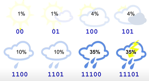
But this is not the case always. Consider the true distribution for those states are not equally likely as follows with the same encoding.
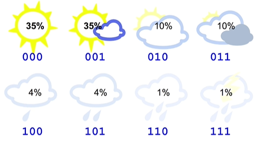
Here, predicted distribution is same () for all the states as we are using same number of bits for all the states. But the true distribution is different. So, entropy and cross entropy would be different.
This is the useful number of bits in this transmission ( on average ). Let's just calculate the actual number of bits that are transmitted on an average, which is cross Entropy.
On an average, we are sending 3 bits of information but only 2.23 bits of information is useful. One more thing that is important to note is that cross entropy is always greater than the entropy. You might ask for proof. But if you think intuitively, when we use more number of bits for the events that are more probable, it will cost us few extra bits, It will be more clear with the following examples.
With this encoding, our cross entropy would be which is close to (entropy). As you have observed, we are still sending additional 0.1 bits of information with this encoding. But it is better than the previous one.
But if we reverse the encoding. i.e., choose more number of bits for more probable events, would result in high cross entropy. For example, take the following encoding.
Here, the average message length or cross-entropy isbits, which is almost twice as the entropy(bits). This is because of the encoding. Here also, we can see that the cross entropy is greater than the entropy by some amount(bits ).
Hence, we can conclude that the cross entropy will always be greater than or equal to entropy. i.e., . OR we can say that the cross entropy is always greater than the entropy by some amount () . The extra information is called relative entropy, or kullback leibler divergence or in general, it is called as KL divergence and is denoted as.
Even though the main topic is cross entropy, we use this is used in several places like building a simple Decision trees, in t-sne ( a dimensionality reduction technique) and even in advanced generative models like Variational Auto Encoders.
But we generally write this in a different formulation which is mostly used to express as a quantity that measures how far the given two distributions are.
where is the true probability distribution and is the predicted probability distribution.
That is all. Now you know what cross entropy is how it is derived from the Information Theory. But it is used quite differently in machine learning. These things doesn't matter when we optimize things. In deep learning, we take true distribution as one-hot representation of the true class label and the predicted probabilities from the model as our predicted probability distribution.
-
Instead of using binary logarithm (base 2), we use natural logarithm( base e). It does not effect as we are just dividing with a constant but it helps while calculating the gradients.
-
For multiclass or multi label classification you might've used categorical cross entropy which is cross entropy. We have n neurons in the final layer for n-class problem.
-
For binary classification, you generally use Binary cross entropy which requires only one neuron in the final layer. You can simply re write the cross entropy with one probability as described in one of the previous sections.
which is also referred as log loss or logistic loss.
References
- A Short Introduction to Entropy, Cross-Entropy and KL-Divergence - Most of the images and the examples are taken from this video. I've tried to simplify it even further along using my own way of explaining things. In the video, I think he went a little faster and people might get confused (well, I did).
- Deep Learning(CS7015): Lec 4.10 Information content, Entropy & cross entropy.