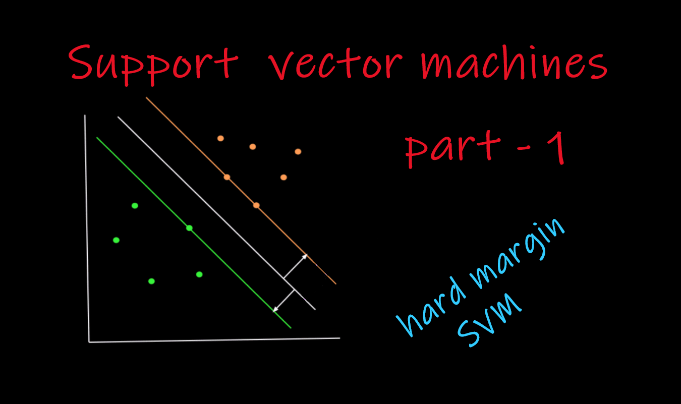
Unlike logistic regression, which tries to find a plane(can be more than one plane that fits the purpose) that separates two set of points in an n-dimensional space, svm tries to find a plane that separates as good as possible.

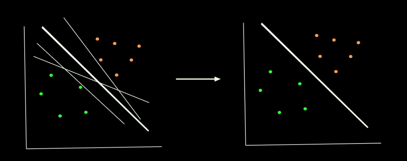
Let's take two set of points that are fully separated with the possible planes that that can separate those two set of points. All the planes (lines) can separate those two set of points. But the thicker plane(line) seems to be the better choice, as it is exactly at the center of the two clusters ( set of points ).

For that we will consider two planes that are parallel to the required plane, one on each side so that the required plane will be exactly at the center of those two planes. The green one passes through through one green point and the other one(orange plane) passes through two orange points. These two planes are in such a way these acts as a decision boundary for that particular class.

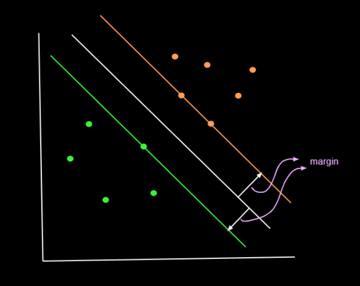
• All the points on and below the green plane are considered as green class.
• And all the points on and above the orange plane are considered as orange class.

So, we will try to find the plane (white one) such that the space between the nearest green and orange point is as large as possible. This space, we call it as margin. Thus svm is called as margin maximization problem. And we have to infer that the plane has to be exactly at the same distance from nearest points from both classes. Otherwise that won't be a perfect plane. Think about it once.

Why bigger margin is better ?

• If we choose a well separating hyperplane, that is close to one class, there is a high chance of misclassification even for very little noise in the test or validation data.
• And intuitively it makes sense.

Before making the optimization function, we need to have a clear idea on equation of a plane, distance from point to plane, and distance between two parallel planes(margin). Here are the resources from which you can understand it better.

Pre-requisites

• Position-vector, line-vector, free-vector and unit-vector
• Linear transformations and matrices | Essence of linear algebra, chapter 3
• Dot products and duality | Essence of linear algebra, chapter 9
• Equation of a plane (3D) from brilliant.org - Same can be applied for 2D. Here, we call that a line. We can also have lines in 3D. But the surface that separates a space into two parts is called line in 2D, plane in 3D, and hyperplane in n-dimensional space.
• Distance from point to plane
  • https://mathinsight.org/distance_point_plane
  • https://mathworld.wolfram.com/Point-PlaneDistance.html

Optimization Function

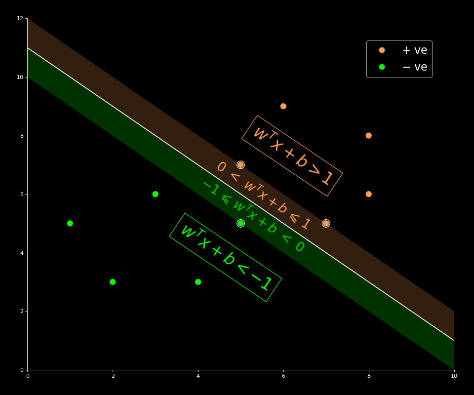
In binary classification problem, we usually have +ve and -ve class points. Here we take orange class as +ve and green as -ve. Unlike logistic regression, we assume the corresponding labels are {-1, 1} instead of 0/1 for -ve and +ve class respectively.

There are so many ways to forming the optimization problem. Here, we will look at the simplest thing possible. While giving the intuition about svm, I told you that that there are two planes which are equidistant from the required plane. Now, forget that those are planes. Instead, think of them like a regions from the decision surface (white plane) on both sides, in which there are no points. All the points, on both sides, lies on and above( or below). So, we need to find a plane that separates two set of points and is equidistant from the nearest points of both the classes. And margin can defined as the distance from the separating plane to the nearest point on both sides.

Let's say that the plane equation is $w^Tx+b=0$. where, $w$ is a weight vector that represent the plane which is normal to the plane and $x$ represents any point on the plane that satisfies the equation (obviously) and $b$ is the bias. Intuitively $w$ decides the orientation of the plane and $b$ decides how far the plane is from the origin. Some say that $b$ is the distance from origin to the plane, It is true if you ignore the sign of the distance. Take a look at this graph to get the better intuition. Feel free to create such planes in a new chart.

The hypothesis is that $\displaystyle w^{T} x_{i} +b >0$ for all +ve points and $\displaystyle w^{T} x_{i} +b<0$ for all -ve points. Here, we want to find a plane that. it is at a equal distance from both nearest negative and nearest positive point(s). Say, $x_n$ is my nearest point. It can be any one of those 3 points(2 orange and 1 green). From any of these points, margin will be same.

Now, If we scale w and b by some constant( k*w and k*b), Does the plane change ? No. The plane remains same. That means we have infinite representations of the same plane. Without the loss of generality, we are assuming that $\displaystyle \ |w^{T}x_{n}+b\ |=1$ for the nearest point(s). It's -1 for the nearest negative class point and +1 for the nearest positive class point to be precise. Instead of taking modulus, we can rewrite the same thing as $\displaystyle \ y_n(w^{T}x_{n}+b)=1$ where $y_n$is the corresponding y label (-1 or +1). It is just the matter of scaling. We are not just assuming things and throwing it away. We will stick to it and try to solve this problem along with this constraint. Let's find the margin.

The distance from $x_n$ (nearest point) to the plane would be $\displaystyle \frac{|w^{T} x_n+b|}{\|w\|}$. We already assumed (constrained) that $\displaystyle |w^Tx_n+b|=1$ for all the nearest points. So, our final margin would be $\displaystyle \frac{1}{\|w\|}$. And the constraint, we will generalize it for all the points. It is exactly $1$ for the nearest points, and $>1$ for other points (which is obvious). we call these as interior points. So we can write this constraint as $y_i(w^Tx_i+b) \geqslant 1$.

Same thing can also be written as follows.

This is constrained optimization problem. This is called as Primal formulation of SVM. We can't solve this directly as we have few constraints. Here, we can use LaGrange to solve it. Essentially, what we will do here is to make the constraint as part of the optimization problem and solve it the usual way. First a quick recap about Lagrange.

Lagrange Duality

The Lagrangian - from khan academy

Feel free to watch the video if you want to get some intuition. But here, We will just discuss how lagrange is used to solve constrained optimization function from svm perspective.

Let's just say we have a function $f(x)$ that we want to minimize and we also have a constraint $g(x)>=0$, then we can write our optimization function as follows.

Here, we have to minimize $f(x)$ and maximize $\alpha$. we call $\alpha$ as Lagrange multiplier and it is always $\geqslant$ 0.

Why $\alpha \geqslant 0$ ?

We are not going to discuss actualities of this. But we can verify whether this is valid or not. Our primary concern is minimizing $f(x)$ w.r.t $x$. In order to have minimum value to our function, the second term in the equation has to be positive. Then only, for whatever $x$, f(x) is minimum, will be the same $x$ for which $\mathcal{L}(x,\alpha)$ is minimum. That means, $\alpha \text{ and }g(x)$ have to be non-negative. Luckily, $g(x) \geqslant 0$ turns out to be our constraint and we improvise for $\alpha$ to be non-negative.

One other way to put this is, Say our constraint is not satisfied for the some $x$, i.e, $g(x)<0$ but $f(x)$ is minimum for that same $x$. Because of the constraint $\alpha \geqslant 0$, we are essentially increasing $\mathcal{L}(x,\alpha)$, which is not what we want. Hope this gives you an intuition on this concept. I think this level of understanding is more than enough. Official name for this is something called as KKT condition. When people mention KKT condition in SVM formulation, you'll know what that is (well, one of the them).

Dual Formulation of SVM

With the current knowledge that we have, we can write our constrained optimization function using lagragian multipliers as follows.

Again, we can't solve it directly because of the constraint on alpha. If there was no such constraint, we could've find optimal $w,b \text{ and } \alpha$ by simply make their gradients as zero or by using some optimization techniques like gradient descent. Instead, we can give this( after some simplification ) to Quadratic Programming libraries they will give us the values. As mentioned, let's try to simplify the equation.

If you observe, there is no constraint on $w$ and $b$. Let's try to find the gradients and make them equal to zero.

After equating them to zero, we derive two important equations and we will be using them later.

Let's try to substitute $w$ in the equation. After this, we will be free of $w \text{ and } b$. This is called Dual formulation of SVM. Time for small exercise. Try to substitute these values in the equation and see if you could derive at the same formulation. Hint: if you have two alphas in the same term, try to separate the $\alpha$'s with a different subscript (say $j$). And, $b$ get's carried away while doing it. So we don't see $b$ anymore. So, the final lagrangian is just has $\alpha$'s. Anyways, here is the final equation.

We are not going to solve this. As mentioned before, we will give this to the QP library, in a nice format. For that, we have to convert this to a minimization problem. We can do that easily by adding a negative condition on it. And we convert this to a format that has matrices instead of variables.

Here, $\alpha, y$ represented as vectors and Q is just a matrix of $y_i's \text{ and }x_i's$ (of size $N \times N$). Given a dataset, all we have to do is construct this matrix, form an equation and give it to QP with the constraints. Here, the constraint for alpha can also be written as $0 \leqslant \alpha \leqslant \infin$.

Finally, we are done with it. You will observe that most of the alphas are actually zeros. Wait, that's not it. Whatever points that we get non-zero values of $\alpha$, are actually the nearest points($x_n$). Once we get $\alpha$'s, we can easily find $w$ as $w=\sum ^{N}_{i=1} \alpha _{i} y_{i} x_{i}$.

why $\alpha=0$ for interior (or non-support vectors)?

• Say, $y_i (w^Tx_i + b) – 1$ is a slack. And we had this KKT condition $\alpha_i(y_i (w^Tx_i + b) – 1)=0 \text{ for } x_i\epsilon \chi$. We already know that for all the interior points (points that are outside of the margin), slack is positive $(>0)$. So, in order to satisfy the KKT condition, $\alpha$ has to be zero.
• And for the support vectors(nearest points), the slack is zero. So, it(QP) can play with the $\alpha$ in order to satisfy the other conditions. As $\alpha\geqslant 0$ is also one of the KKT conditions we have to satisfy, the values of $\alpha$ could only be positive wherever possible.

Now, $w$ only depends on the nearest points (as $\alpha=0$ for the remaining(interior) points). So these are called Support Vectors and hence the name Support Vector Machines. Amazing isn't it. Before you get too happy, we still have to find $b$. For that, we have to go to where it all began. I mean, the optimization. Remember we had the assumption that $y_n(w^Tx_n+b)=1$ for nearest points (support vectors). Just take any support vector and we can have our $b$. Yes, take any support vector, It will come as same. Everything seems connected and makes sense right. Don't worry even if you have a slightest doubt, we have all the proof we need to prove it.

SVM from sklearn

Now, let's verify this theory with implementation of SVM in sklearn (scikit learn). In sklearn, we can do classification using support vector machines using 3 different classes(python classes). We will use SVC (support vector classifier).

Whatever we have learned, we call this as Hard Margin SVM. Till now, we haven't considered the case where the points are not perfectly separable. In such cases we allow few errors to happen and we call this as Soft Margin SVM. We use some parameter $C$ to tune it, which is mandatory in sklearn. In order to mimic the hard-margin svm, we have to keep $C$ as large as possible. More on this parameter later.

One more concept is kernel. There is something called kernelization in SVM, where we can replace $x_i^Tx_j$ with some value which we get by combining $x_i$ and $x_j$. Again, more on that later. For now, to mimic this simple case of svm, we keep kernel as linear and $C$ as $1000$. That means, we are doing hard margin svm.

First, let's create some data. I have created some sample dataset that is close to what we have seen in the example figure. And we will apply svm on it.

import numpy as np
from sklearn import svm

# create the dataset
X = np.array([[2, 3],[1, 5],[3, 6],[5, 5],[4, 3],
              [7, 5],[5, 7],[8, 6],[8, 8],[6, 9]])
y = np.array([0, 0, 0, 0, 0,
              1, 1, 1, 1, 1])

# Train the model
clf = svm.SVC(kernel='linear', random_state=25)
clf.fit(X, y)

I kept the labels as $0$'s and $1$'s just because it is easy to plot. Sklearn will automatically takes $1$ as positive class($+1$) and $0$ as negative class($-1$) and classify accordingly. Now, let's draw a decision boundary. so that we can clearly see the margin and the support vectors which are on the margin. And feel free to skip the code. Mostly, this code is taken from sklearn documentation.

with plt.style.context('dark_background'):  # just to make the background black
    fig = plt.figure(num=None, figsize=(12, 10), dpi=80, facecolor='w')
    # set the x-axis and y-axis limits
    plt.xlim(0,10)
    plt.ylim(0,12)
    
    # plot data
    scatter = plt.scatter(X[:,0], X[:,1], c=y, cmap=colormap, s=100)
    plt.legend(handles=scatter.legend_elements()[0][::-1], labels=['$+$ ve', '$-$ ve'],
               fontsize=20, markerscale=1.6,borderaxespad=2)
    # ########### decision function ########### #
    ax = plt.gca()  # get_current_axes
    # create grid of points
    xx = np.linspace(ax.get_xlim()[0]+1, ax.get_xlim()[1]-1, 30)
    yy = np.linspace(ax.get_ylim()[0]+1, ax.get_ylim()[1]-1, 30)
    YY, XX = np.meshgrid(yy, xx)
    xy = np.vstack([XX.ravel(), YY.ravel()]).T
    
    # find the decision function output for those grid of points
    Z = clf.decision_function(xy).reshape(XX.shape)
    # plot decision boundary (where decision function outputs are -1,0 or 1)
    # which are margins.
    colors=[(0, 1, 0, 1.0),(1,1,1,1),(1, 0.61, 0.33, 1.0)]
    ax.contour(XX, YY, Z, colors='w', levels=[0],
               linestyles=['-'])
    colors=[(0, 1, 0, 0.2),(1,1,1,0),(1, 0.61, 0.33, 0.2)]
    ax.contourf(XX, YY, Z, colors=colors, levels=[-0.99, -0.01, 0.01, 0.99])

    # plot support vectors
    ax.scatter(clf.support_vectors_[:, 0], clf.support_vectors_[:, 1], s=200,
               linewidth=1, facecolors='none', edgecolors='white')
    
    # save figure
    plt.tight_layout(pad=3)
    ax.spines['top'].set_visible(False)
    ax.spines['right'].set_visible(False)
    fig.patch.set_facecolor("black")
    
    orange_interior = (1, 0.61, 0.33, 1.0)
    plt.annotate(s="$w^Tx+b>1$", xy=(5.2,6.3), fontSize=30,  rotation=-34,
                 color=orange_interior, bbox=dict(facecolor='none', edgecolor=orange_interior, pad=10))
    plt.annotate(s=r"$0\ <\ w^Tx+b\ \leqslant\ 1$", xy=(4.35,4.8), fontSize=24,  rotation=-34,
                 color=(1, 0.61, 0.33, 1))
    plt.annotate(s=r"$-1\ \leqslant\ w^Tx+b\ <\ 0$", xy=(4,4), fontSize=24,  rotation=-34,
                 color=(0, 0.8, 0, 1.0))
    green_interior = (0, 1, 0, 1.0)
    plt.annotate(s=r"$w^Tx+b<-1$", xy=(3.5,2.7), fontSize=30,  rotation=-34,
                 color=green_interior, bbox=dict(facecolor='none', edgecolor=green_interior, pad=10))
    
    plt.savefig("linear_SVM.png", dpi=80)

    plt.show()

The main things that we have to focus on here are decision function and margin. Decision function is nothing but $w^Tx_q+b$. where, $x_q$ is any given query point. Based on the sign, we decide it's class label. i.e., The class of $x_q$ is negative of the decision function output is negative and positive if the output is positive. This is the hypothesis remember?

And we also assumed that for all the nearest points, the decision function is either $-1$ or $1$ (depends on the class). So, we just draw those contour lines. As expected, the support vectors would be on those contour lines.

The main thing that we have to take from the plot are follows.

• $\alpha=0$ for all the interior points, on both negative and positive side. i.e., non-support vectors(which are outside the shaded region). And $\alpha>0$ for all the support vectors ( which are on the edge of the shaded regions OR which are on the edge of margin on both sides).
• $0<w^Tx_q+b\leqslant1$ for points which are in the marginal region(boundary included) on positive side, i.e., light-orange shaded region and $-1<=w^Tx_q+b<0$ for the points which lies in the marginal region(boundary included) on the negative side of the plane, i.e light-green shaded region.
• $w^Tx_q+b>1$ for all the points above the positive marginal region(boundary excluded) and $w^Tx_q+b<-1$ for all the points that are below the negative marginal region(boundary excluded).

Let's verify few things. Here, clf is the classifier that we have trained earlier.

• Support vectors

  # indices of support vectors w.r.t to our input data
  clf.support_
  # OR, get support vectors (points) directly
  clf.support_vectors_  # same as X[clf.support_]
  
  # Output: array([[5, 5],[7, 5],[5, 7]]),
  

• Dual Coefficients

  • Sklearn does not give $\alpha$'s directly. Instead, we can get $\alpha_ny_n$ and that too only for support vectors. For other points, it is anyway zero. We will also verify the condition $\sum_i^N \alpha_iy_i=0$.

  print(clf.dual_coef_)
  # Out: array([[-1. ,  0.5,  0.5]])
  
  # verify alpha_n*y_n satisfies 
  assert clf.dual_coef_.sum()==0
  

  Each value in this array corresponds to each support vector that we got previously.

  • weight vector and intercept ($w$ and $b$)

  • Weight vector from the equation $\boxed{w=\sum ^{N}_{i=1} \alpha _{i} y_{i} x_{i}}$. And we already know that $\alpha$ for non-support vectors are zero. We also discussed why is it so. Anyways, we only get the dual coefficients ($\alpha_iy_i$) for support vectors and It should be easy for us to get the $w$. And one more thing is, we also have clf.coef_ and clf.intercept which are valid only if the kernel is linear (in this case).

    # weight vector (w)
    w = clf.dual_coef_.dot(clf.support_vectors_)
    print(w, clf.coef_,np.allclose(w, clf.coef_))
    # Output: [[1. 1.]] [[1. 1.]] True
    
    
    # bias or intercept (b)
    for i in range(len(clf.support_vectors_)):
        sv_index = clf.support_[0]
        point = X[sv_index]
        label=y[sv_index] if y[sv_index]==1 else -1
        b = (1/label) - clf.dual_coef_.dot(clf.support_vectors_).dot(point)
        print(b, clf.intercept_, np.allclose(clf.intercept_,b))
    # output: [-11.] [-11.] True
    #               [-11.] [-11.] True
    #               [-11.] [-11.] True
    

    For the intercept, as we said earlier, we are checking for every support vector just to prove the point that we get same $b$ for every support vector. And we are also changing the label to {-1, 1}.

• Decision Function ($w^Tx_q+b$) :

  • Now, given a query point, we are just verifying whether the decision function that we assumed in the beginning. If the decision function output is negative, then we say that $x_q$ is $-ve$ and $+ve$ if the decision function output is positive.

  • We will take a point in the lower region. Let's just say the point is $(2,4)$. We should get negative value.

    point = np.array([[2,4]])
    decision_output = np.dot(clf.coef_, point.T) + clf.intercept_  # w^Tx+b
    
    # verifying from sklearn function
    np.allclose(clf.decision_function(point), decision_output)
    # Output: [[-5.]] True
    

Pheww. I think this is enough for one blog. In this we learned how can we form an optimization function to obtain maximum margin between two set of points and few other things ( actually, a lot of things). I know you still have few questions. I hope those will be answered too. I hope these two are in the set of questions that you have in your mind.

• What if our data is not perfectly separable?
• What is kernelization in SVM and why it is powerful?
• And last but not least, what is hinge loss ?

Excited..! Me too. Hasta luego amigas y amigos..! Have a good day : )